AUTOMATIC DIFFERENTIAON (Part 1)

1. Introduction

At the heart of Decision Science lies the pivotal concept of Optimization, a critical tool for analysis and forecasting in various domains, especially in the domain of financial markets. Problems like Portfolio Optimization, Option Pricing, and optimal control in scenarios (like Asset Pricing and continuous-time Portfolio Optimization) frequently translate into numerical optimization problems. These problems invariably demand the computation of derivatives to arrive at solutions.

Numerical derivatives play a key role in identifying extrema of functions and are commonly categorized as follows:

1. Gradients: Providing the direction of steepest ascent or descent for a scalar function.
2. Jacobians: Extending gradients to vector-valued functions, indicating the sensitivity of each output component to changes in inputs.
3. Hessians: Going a step further, these involve second derivatives and describe the curvature of a function’s surface.

Computation of this derivatives in computer programs can be classified into four categories.

1. Manually working out deriviatives and coding them.
2. Numerical differentiation
3. Symbolic differentiation- using expression manipulation in computer algebra systems.
4. Automatic differentiation.

In financial market analysis, optimization problems often revolve around refining predictions, minimizing errors, or maximizing certain outcomes. These problems can be distilled into finding pathways that enhance performance. Achieving this frequently involves adjusting model parameters in the direction that maximally improves performance. This optimal direction is arrived at by differentiating the performance surface with respect to the model parameters.

However, the process of calculating derivatives encounters several obstacles:

1. Complex Operations Chain: Performance measures are often the result of intricate operations woven into complex algorithms.
2. High-Dimensional Parameters: Performance functions frequently depend on an extensive array of parameters, leading to high-dimensional derivative calculations.

Automatic Differentiation (AD) emerges as a promising technology which offers software solutions for the automated computation of derivatives for general functions. It not only expedites the process of obtaining derivatives but also sheds light on the underlying landscape of performance surfaces, aiding decision-makers in navigating the complexities of financial market analysis.

2. Automatic differentiation :Unveiling the Chain Rule’s Power

Automatic differentiation is a chain rule based technique for evaluating the derivatives with respect to the input variables of functions it uses the chain rule to break long calculations into small pieces,each can be easily differentiated.

The chain rule tells us how to combine the differentiated pieces into the overall deriviative for example given the following function

\[f(x,y) = 2xy\]

we can set \(v = xy\) and obtain the partial deriviative with respect to \(x\) by the chain rule \(\frac{\partial f}{\partial x} = \frac{\partial f}{\partial v} . \frac{\partial v}{\partial x} = 2y\)

The final value multiplies the two component derivatives,\(\frac{\partial f}{\partial v} = 2\) and \(\frac{\partial v}{\partial x} = y\).To use this pieces as part of a longer calculation,we substitute the numerical value of y and store only that numerical value.E.g if \(y = 0.1\) then \(\frac{\partial f}{\partial x}=0.2\)

In essence, intricate calculations can be deconstructed into a series of elementary steps. At each juncture, we compute the numeric value of the component derivative, fuse it with preceding component values, and store the resultant numeric outcome for subsequent steps. This streamlined approach requires storing only a modest amount of information while progressively combining component values to derive the final outcome. While the theoretical accuracy remains on par with symbolic derivatives, the incorporation of numeric values accelerates the process and minimizes computational storage requirements.

2.1 Evaluation traces: Simplifying Complex Functions

To decompose functions into elementary steps,the construction of evaluation traces is necessary.Let’s explore another example function \(f:\mathbb{R}^n\xrightarrow{} \mathbb{R}^m\)

\(y=[sin(x_1/x_2) + x_1/x_2 - exp(x_2)][x_1/x_2 - exp(x_2)]\) we proceed to define the following variables:

• \(v_{i-n} = x_i,i = 1,..,n\) are the input variables,

• \(v_i,i=1,..,l\) for the intermediate variables

• \(y_{m-i} = v_{l-i},i=m-1,...,0\) for the output variables.

let’s evaluate the function when \(x_1=1.5\) and \(x_2=0.5\) and record all the intermediate values

Intermediate Vars	Expressions	Values
\(V_{-1}\)	\(x_1\)	1.5
\(V_{0}\)	\(x_2\)	0.5
\(V_{1}\)	\(x_1/v_0\)	3.000000
\(V_{2}\)	\(\sin(v_1)\)	0.1411
\(V_{3}\)	\(\exp(v_0)\)	1.6487
\(V_{4}\)	\(V_1 - V_3\)	1.3513
\(V_{5}\)	\(V_2 - V_4\)	1.4924
\(V_{6}\)	\(V_5 \cdot V_4\)	2.0167

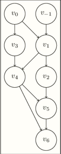
Here,\(V_6\) represents the final output variable \(y\) which equals to \(2.0167\). This process can be visually represented with the variables forming nodes in a graph and the edges represent the algebraic relationships.

It’s important to establish initial conditions for the derivatives as a starting point for the differentiation process. These initial values act as the foundation for the differentiation process. Moving forward, calculating the derivatives of \(f\) with respect to \(x_1\) and \(x_2\) involves following the evaluation trace and computing the derivatives for each intermediate variable step by step. This path leads us to the forward mode automatic differentiation algorithm.

2.2 Forward mode Automatic differentiation

Forward mode automatic differentiation (AD) is a technique that breaks down complex expressions into a sequence of differentiable elementary operations. This method is especially useful when we want to calculate derivatives of functions with respect to multiple input variables. Let’s explore this concept through another example:

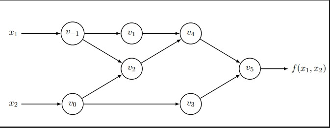
Example: Consider the function \(f(x_1,x_2) = cos(x_1) + x_1exp(x_2)\).We can divided this expression into elementary operations for a systematic evaluation:

\(w_1 = x_1\) \(w_2 = x_2\) \(w_3 = exp(w_2)\) \(w_4 = w_1 . w_3\) \(w_5 = cos(w_1)\) \(w_6 = w_4 + w_5\) \(f(x_1,x_2) = w_6\)

Computational graph

Now, let’s move on to finding the derivatives using differentiation rules and applying the chain rule to each elementary operation. This will allow us to compute the derivatives of each intermediate variable and ultimately the derivative of the function:

\[w'_{1} = \text{seed} \in \{0, 1\}\] \[w'_{2} = \text{seed} \in \{0, 1\}\] \[w'_{3} = exp(w_2)w'_2\] \[w'_{4} = w'_1w_3 + w_1w'3\] \[w'_{5} = -sin(w_1)w'_1\] \[w'_{6} = w'_4 + w'_5\] \[f'(x_1,x_2) = w'_6\]

Efficiency and Applicability:

One significant advantage of forward mode AD is that only one sweep is necessary to compute derivatives for functions like \(f:\mathbb{R}\xrightarrow{} \mathbb{R}^m\).This makes the method efficient for scenarios where \(m >> 1\).However forward mode AD might not perfom as well for functions \(f:\mathbb{R}^n\xrightarrow{} \mathbb{R}\) .In terms of complexity,the method’s order is \(O(n)\) where n is the dimension of the input vector.

3. Using Dual Numbers

Dual numbers introduce a unique mathematical construct by extending real numbers with a new element \(\epsilon\) that follows the rule \(\epsilon^2 = 0\). Mathematically,a dual number can be represented as \(\alpha + b\epsilon\).where α and b are real numbers. Dual numbers follow familiar addition and multiplication rules:

• Addition : \((a + b\epsilon) + (c + d\epsilon) = (a + c)+(b + d)\epsilon\)

• Multiplication:\((a + b\epsilon)(c + d\epsilon) = ac + (ad + bc)\epsilon + db\epsilon^2 = ac + (ad + bc)\epsilon\)

The connection between dual numbers and differentiation becomes clear when considering the Taylor series Expansion.For an arbitrary real function \(f:\mathbb{R}\xrightarrow{}\mathbb{R}\) its Taylor series expansion at \(x_0\) is given by: \(f(x) = f(x_0) + f'(x_0)(x - x_0)+..+ \frac{f^{(n)}(x_0)}{n!}(x - x_0)^n + O((x - x_0)^{n+1})\)

Using dual numbers as inputs,the expansion simplifies to: \(f(x) = f(x_0) + f'(x_0)x_1\epsilon\)

Here, higher-order terms vanishes due to \(\epsilon^2 = 0\).Thus, the derivative of a real function can be precisely calulated exactly by evaluating the function using dual numbers and taking the \(\epsilon \text{component} f_1\) of the results as \(f(x_0 + \epsilon) = f(x_0) + f'(x_0)\epsilon.\)

As opposed to numerical differentiation methods calculating the derivatives with dual numbers does not introduce an error by truncating the Taylor expansion.Therefore the necessity to find an optimal step size is eliminated and we can simply choose \(x_1 = 1\)

Illustration.

Let’s consider the function \(f(x) = 3x + 2\)

Evaluated at \(x = 4\) using dual numbers we have:

\[f(4 + 1\epsilon) = (4 + 1\epsilon)*(3 * 0\epsilon) + (2 + 0\epsilon)\] \[12 + 3\epsilon + 0\epsilon+ 0\epsilon^2 + 2 + 0\epsilon = 14 + 3\epsilon\]

References

• https://www.educative.io/answers/what-is-forward-mode-differentiation
• https://liqimai.github.io/blog/Forward-Automatic-Differentiation/
• https://www.frontiersin.org/articles/10.3389/fevo.2022.1010278/full
• https://arxiv.org/abs/1502.05767
• https://doi.org/10.48550/arXiv.1910.07934